Advertising Effectiveness Analysis • activecampaignr

Overview

This vignette shows how to combine ActiveCampaign deal data with daily advertising spend to calculate:

Cost per lead (CPL) — how much you spend to generate one new deal
Cost per sale (CPS) — how much you spend to close one deal
Lead-to-sale velocity — how many days from deal creation to won
Windowed attribution — which week’s ad spend drove which week’s sales

Setup

library(activecampaignr)
library(dplyr)
library(tidyr)
library(ggplot2)

ac_auth_from_env()

Step 1: Pull Deal Data

# Fetch deals — cdate/mdate are already POSIXct, value is already numeric
deals <- ac_deals()

# Select the columns we need
# status is returned as character: "0" = open, "1" = won, "2" = lost
deal_dates <- deals |>
  transmute(
    deal_id = id,
    created = as.Date(cdate),
    closed = as.Date(mdate),
    status = status,
    value = value
  )

# Won deals with velocity
won <- deal_dates |>
  filter(status == "1") |>
  mutate(
    days_to_close = as.integer(closed - created)
  )

Step 2: Prepare Your Ad Spend Data

Create a CSV with your daily advertising spend. The file needs two columns: date and spend.

date,spend
2025-01-01,150.00
2025-01-02,200.00
2025-01-03,175.50
...

You can export this from Google Ads, Meta Ads Manager, or any platform. If you run multiple channels, either sum them into one spend column or add a channel column for per-channel analysis.

# Load your spend data
spend <- read.csv("daily_spend.csv") |>
  mutate(date = as.Date(date))

Step 3: Daily Leads and Sales

# Count new leads (deals created) per day
daily_leads <- deal_dates |>
  count(date = created, name = "leads")

# Count won deals per day
daily_sales <- won |>
  count(date = closed, name = "sales")

# Revenue per day
daily_revenue <- won |>
  group_by(date = closed) |>
  summarise(revenue = sum(value / 100, na.rm = TRUE), .groups = "drop")

# Combine into one daily table
daily <- spend |>
  full_join(daily_leads, by = "date") |>
  full_join(daily_sales, by = "date") |>
  full_join(daily_revenue, by = "date") |>
  replace_na(list(spend = 0, leads = 0, sales = 0, revenue = 0)) |>
  arrange(date)

Step 4: Cost per Lead and Cost per Sale

Simple daily metrics

daily_metrics <- daily |>
  mutate(
    cpl = if_else(leads > 0, spend / leads, NA_real_),
    cps = if_else(sales > 0, spend / sales, NA_real_),
    roas = if_else(spend > 0, revenue / spend, NA_real_)
  )

daily_metrics |>
  filter(!is.na(cpl)) |>
  summarise(
    median_cpl = median(cpl),
    median_cps = median(cps, na.rm = TRUE),
    median_roas = median(roas, na.rm = TRUE)
  )

Weekly rollup (more stable)

Daily metrics are noisy. Weekly aggregation smooths out day-of-week effects and small sample sizes.

weekly <- daily |>
  mutate(week = floor_date(date, "week")) |>
  group_by(week) |>
  summarise(
    spend = sum(spend),
    leads = sum(leads),
    sales = sum(sales),
    revenue = sum(revenue),
    .groups = "drop"
  ) |>
  mutate(
    cpl = if_else(leads > 0, spend / leads, NA_real_),
    cps = if_else(sales > 0, spend / sales, NA_real_),
    roas = if_else(spend > 0, revenue / spend, NA_real_)
  )

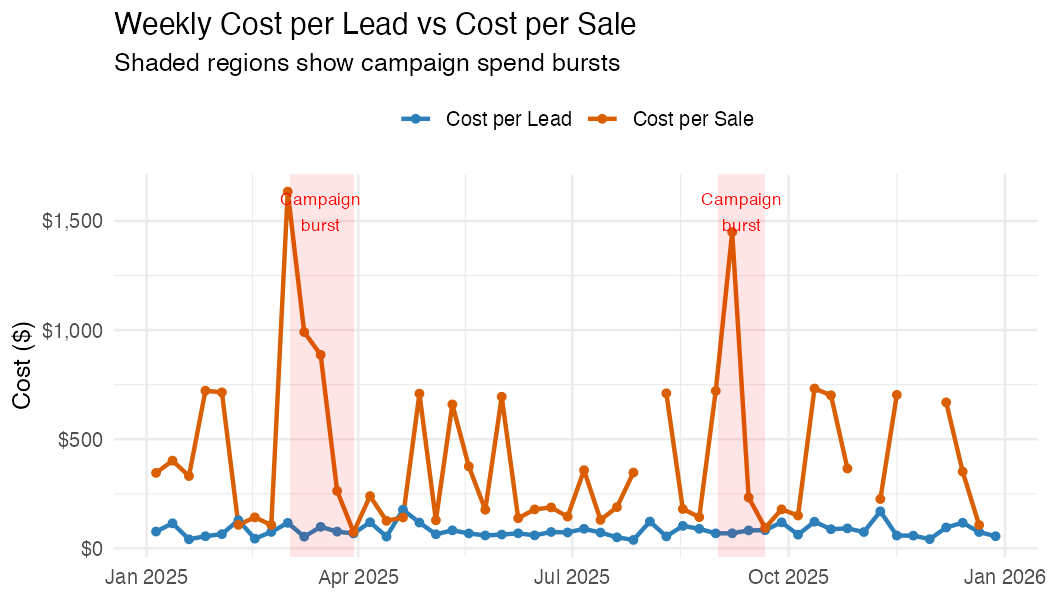
weekly

Plot: Weekly CPL and CPS

weekly |>
  select(week, cpl, cps) |>
  pivot_longer(-week, names_to = "metric", values_to = "cost") |>
  ggplot(aes(week, cost, colour = metric)) +
  geom_line(linewidth = 1) +
  geom_point() +
  scale_y_continuous(labels = scales::dollar) +
  labs(
    title = "Weekly Cost per Lead vs Cost per Sale",
    x = NULL, y = "Cost ($)", colour = NULL
  ) +
  theme_minimal()

Example output (synthetic data):

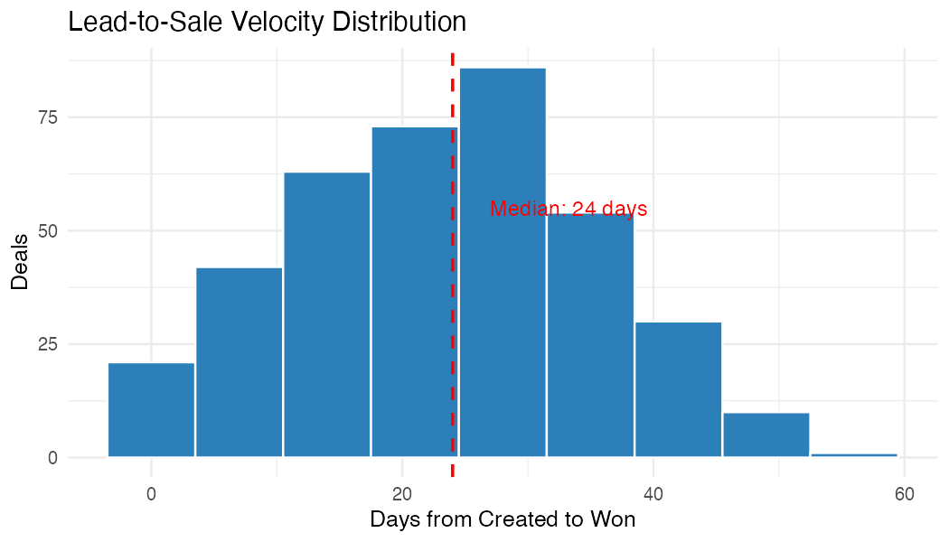
Step 5: Lead-to-Sale Velocity

Understanding how long it takes to convert a lead to a sale is critical for windowed attribution. If your average velocity is 3 weeks, then this week’s sales were driven by ad spend from 3 weeks ago.

# Velocity distribution
velocity_summary <- won |>
  summarise(
    deals = n(),
    median_days = median(days_to_close),
    mean_days = round(mean(days_to_close), 1),
    p25_days = quantile(days_to_close, 0.25),
    p75_days = quantile(days_to_close, 0.75)
  )

velocity_summary

ggplot(won, aes(days_to_close)) +
  geom_histogram(binwidth = 7, fill = "#2c7fb8", colour = "white") +
  geom_vline(
    xintercept = median(won$days_to_close),
    linetype = "dashed", colour = "red"
  ) +
  labs(
    title = "Lead-to-Sale Velocity Distribution",
    subtitle = paste("Median:", median(won$days_to_close), "days"),
    x = "Days from Created to Won", y = "Deals"
  ) +
  theme_minimal()

Example output (synthetic data):

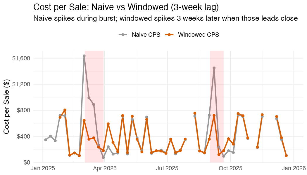
Step 6a: Windowed Attribution (Aggregate)

Naive CPS divides this week’s spend by this week’s sales. But if your median velocity is 3 weeks, this week’s sales were actually driven by spend from 3 weeks ago. This matters when spend varies over time.

Consider a campaign burst: you double your ad budget in March. Naive CPS spikes in March (high spend, same number of sales closing). Windowed CPS stays flat in March but spikes 3 weeks later, when the leads generated by that burst actually close. This gives you a more accurate picture of what each sale really cost.

If your spend is steady week-to-week, the two lines will overlap because lag(spend, 3) ≈ spend. The divergence only appears when spend has meaningful variation (campaign bursts, budget changes, seasonal ramps).

lag_weeks <- round(median(won$days_to_close) / 7)

windowed <- weekly |>
  mutate(
    # Shift spend back by the median velocity
    lagged_spend = lag(spend, n = lag_weeks),
    # Windowed CPS: this week's sales attributed to spend N weeks ago
    windowed_cps = if_else(
      sales > 0 & !is.na(lagged_spend),
      lagged_spend / sales,
      NA_real_
    ),
    windowed_roas = if_else(
      !is.na(lagged_spend) & lagged_spend > 0,
      revenue / lagged_spend,
      NA_real_
    )
  )

Compare naive vs windowed

windowed |>
  select(week, naive_cps = cps, windowed_cps) |>
  pivot_longer(-week, names_to = "method", values_to = "cost") |>
  ggplot(aes(week, cost, colour = method)) +
  geom_line(linewidth = 1) +
  geom_point() +
  scale_y_continuous(labels = scales::dollar) +
  labs(
    title = paste0(
      "Cost per Sale: Naive vs Windowed (", lag_weeks, "-week lag)"
    ),
    x = NULL, y = "Cost per Sale ($)", colour = NULL
  ) +
  theme_minimal()

Example output (synthetic data with campaign bursts in March and September):

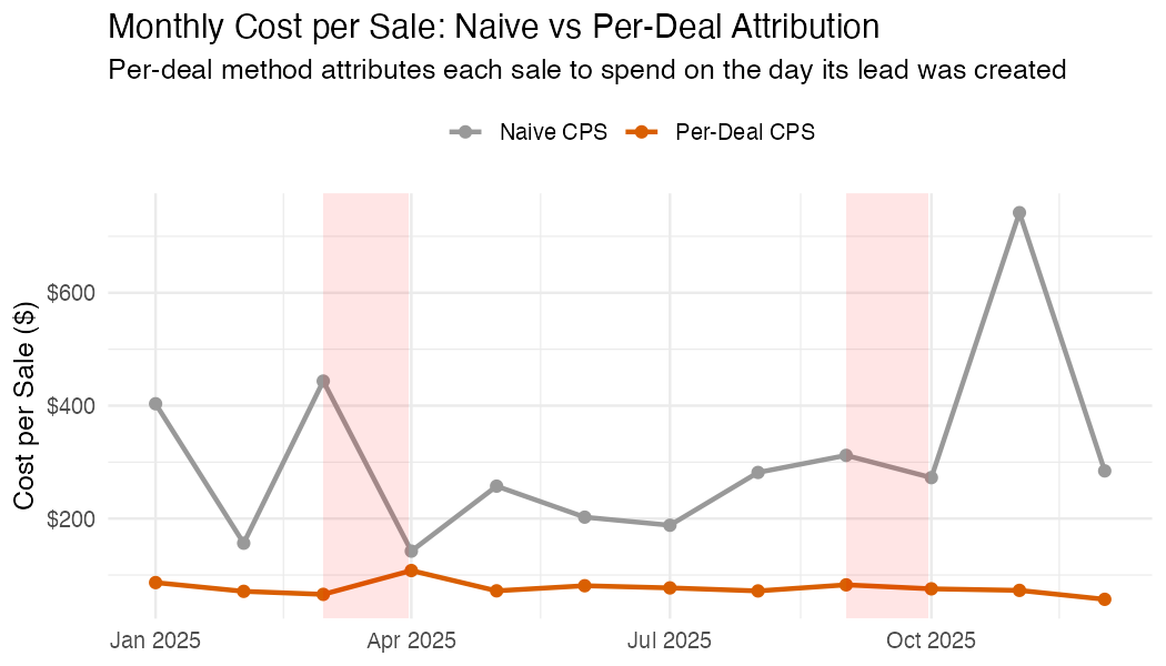
Step 6b: Per-Deal Attribution

The windowed approach above is an aggregate approximation. For more precise attribution, work at the deal level: for each won deal, look up the ad spend on the day that deal was created, then divide by the number of leads created that same day. This gives each deal its own attributed acquisition cost.

Deal 1042: created 10 Mar, closed 2 Apr (23 days)
  Ad spend on 10 Mar: $280
  Leads created on 10 Mar: 4
  → Attributed cost for deal 1042: $280 / 4 = $70

This method handles uneven spend naturally. A deal created during a campaign burst gets a higher attributed cost than one created on a quiet day, regardless of when it closes.

# For each won deal, look up spend on the day it was created
won_attributed <- won |>
  left_join(
    daily |> select(date, daily_spend = spend, daily_leads = leads),
    by = c("created" = "date")
  ) |>
  mutate(
    # This deal's share of that day's spend
    attributed_cost = if_else(
      daily_leads > 0,
      daily_spend / daily_leads,
      NA_real_
    )
  )

# Summary: what did each sale actually cost to acquire?
won_attributed |>
  filter(!is.na(attributed_cost)) |>
  summarise(
    deals = n(),
    median_cost = median(attributed_cost),
    mean_cost = mean(attributed_cost),
    p25 = quantile(attributed_cost, 0.25),
    p75 = quantile(attributed_cost, 0.75)
  )

Compare naive vs per-deal CPS over time

# Monthly comparison
monthly_attributed <- won_attributed |>
  mutate(month = floor_date(closed, "month")) |>
  group_by(month) |>
  summarise(
    avg_attributed_cps = mean(attributed_cost, na.rm = TRUE),
    .groups = "drop"
  )

monthly_naive <- daily |>
  mutate(month = floor_date(date, "month")) |>
  group_by(month) |>
  summarise(spend = sum(spend), sales = sum(sales), .groups = "drop") |>
  mutate(naive_cps = if_else(sales > 0, spend / sales, NA_real_))

monthly_attributed |>
  left_join(monthly_naive |> select(month, naive_cps), by = "month") |>
  select(month, `Naive CPS` = naive_cps, `Per-Deal CPS` = avg_attributed_cps) |>
  pivot_longer(-month, names_to = "method", values_to = "cost") |>
  ggplot(aes(month, cost, colour = method)) +
  geom_line(linewidth = 1) +
  geom_point(size = 2) +
  scale_y_continuous(labels = scales::dollar) +
  labs(
    title = "Monthly Cost per Sale: Naive vs Per-Deal Attribution",
    subtitle = "Per-deal attributes each sale to spend on the day its lead was created",
    x = NULL, y = "Cost per Sale ($)", colour = NULL
  ) +
  theme_minimal()

Example output (synthetic data with campaign bursts in March and September):

Which method to use?

Method	Pros	Cons
Naive (same-period)	Simple, no assumptions	Conflates cause and effect
Windowed (lagged)	Accounts for velocity	Uses median lag for all deals; loses deal-level detail
Per-deal attribution	Most accurate; handles variable spend and velocity	Requires deal-level created dates; assumes all leads come from paid ads

For most teams, start with per-deal attribution. Fall back to windowed if you don’t have reliable deal creation dates.

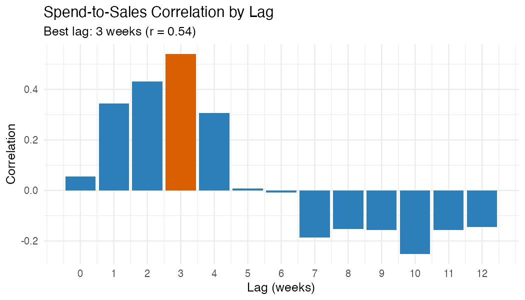
Step 7: Spend-to-Sales Correlation

Test which lag window produces the strongest correlation between spend and sales. This helps validate your assumed velocity.

# Test lags from 0 to 12 weeks
lag_test <- tibble(lag_weeks = 0:12) |>
  rowwise() |>
  mutate(
    correlation = cor(
      weekly$spend[1:(nrow(weekly) - lag_weeks)],
      weekly$sales[(1 + lag_weeks):nrow(weekly)],
      use = "complete.obs"
    )
  ) |>
  ungroup()

best_lag <- lag_test |> slice_max(correlation, n = 1)

ggplot(lag_test, aes(lag_weeks, correlation)) +
  geom_col(fill = "#2c7fb8") +
  geom_col(
    data = best_lag,
    fill = "#d95f02"
  ) +
  labs(
    title = "Spend-to-Sales Correlation by Lag",
    subtitle = paste0(
      "Best lag: ", best_lag$lag_weeks,
      " weeks (r = ", round(best_lag$correlation, 2), ")"
    ),
    x = "Lag (weeks)", y = "Correlation"
  ) +
  theme_minimal()

Example output (synthetic data):

Step 8: Summary Table

summary_table <- tibble(
  metric = c(
    "Total ad spend",
    "Total leads generated",
    "Total sales closed",
    "Total revenue",
    "Cost per lead (CPL)",
    "Cost per sale (CPS)",
    "Return on ad spend (ROAS)",
    "Median lead-to-sale velocity",
    "Best spend-to-sale lag"
  ),
  value = c(
    scales::dollar(sum(daily$spend)),
    format(sum(daily$leads), big.mark = ","),
    format(sum(daily$sales), big.mark = ","),
    scales::dollar(sum(daily$revenue)),
    scales::dollar(sum(daily$spend) / max(sum(daily$leads), 1)),
    scales::dollar(sum(daily$spend) / max(sum(daily$sales), 1)),
    paste0(round(sum(daily$revenue) / max(sum(daily$spend), 1), 1), "x"),
    paste(median(won$days_to_close), "days"),
    paste(best_lag$lag_weeks, "weeks")
  )
)

summary_table

Adapting This Analysis

Multiple ad channels

If your spend CSV includes a channel column (e.g., Google, Meta, LinkedIn), group by channel throughout:

weekly_by_channel <- daily |>
  mutate(week = floor_date(date, "week")) |>
  group_by(week, channel) |>
  summarise(across(c(spend, leads, sales, revenue), sum), .groups = "drop")

Pipeline-specific analysis

Filter deals by pipeline to analyse specific products:

# Only deals from pipeline "1" (e.g., your main sales pipeline)
deals <- ac_deals(pipeline = "1")

Using deal won dates from activity logs

AC’s mdate is the last-modified date, not necessarily the won date. For more accurate velocity, use ac_deal_won_dates() to extract the actual status-change timestamp from deal activity logs:

won_dates <- ac_deal_won_dates(won$deal_id)
won <- won |>
  left_join(won_dates, by = c("deal_id" = "deal_id")) |>
  mutate(
    closed = coalesce(as.Date(won_date), closed),
    days_to_close = as.integer(closed - created)
  )